¶ Summary
- The case involves optimizing a financial contract — specifically, a "knock-in knock-out equity accumulator" — a machine that triggers daily buy or sell orders for a stock based on algorithmic trading rules within a time window. The key challenge is to identify trading rule parameters that maximize profit while strictly meeting capital requirements and risk constraints. Although calculating the NPV distribution for a single rule set is relatively fast (i.e. one minute in our case), exhaustively testing multiple combinations through trial-and-error is computationally intensive and can take hours.
- The goal is to accelerate the search for trading rule combinations that optimize profit while ensuring compliance with capital and risk constraints, and to achieve this with minimal modification to the existing codebase.
- The task is to develop code for analyzing the stock’s historical volatility (descriptive analytics) and to run thousands of NPV predictions under different trading rule scenarios (predictive analytics). Additionally, the goal includes modifying the code to enable parallel execution and deploying the solution on scalable cloud infrastructure — all while minimizing changes to the existing codebase. Trading rules are parameterized for iterative testing, with each configuration evaluated against risk metrics (e.g., Roy’s SFRatio). A parallel computing framework, selected for minimal code changes, is deployed on scalable cloud infrastructure to accelerate the process. The recommended configuration (prescriptive analytics) the one that, in simulation, yields the highest profit.
- The approach enables rapid exploration of trading strategies, cutting down optimization time from many hours to a fraction, while maintaining compliance and maximizing profitability potential.
¶ Process and context
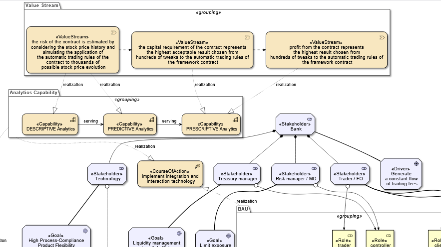
→ Process and context Archimate model
¶ Methodology used
We present the project execution in accordance with the CRISP-DM framework .
¶ The business issue
¶ Background
We want to setup an environment for the definition of an equity derivative financial contract based on user-defined 'draft' rules and we want to finalize those rules through a simulation model.
¶ Objectives and success criteria
We want our simulations to identify the set of hardcoded algorithmic trading rules that minimize the shortfall risk.
¶ Requirements, Assumptions, and Constraints
¶ Key financial assumptions and limits of the pricing function
The "profit" calculation implemented in our program is going to be a simplified one. The main limitations and assumptions are:
- fixed drift and volatility of the future underlying prices
- future drift and volatility = past drift and volatility
- macroeconomic context: future = past
- no dividends in the underlying
- no stock splits
- no discounting
- the KPI is the accounting P/L
- the implemented algo only supports closing prices - no candlesticks, no moving averages
- no public holidays in the simulated future prices
- unlimited treasury funding (...)
- no brokerage fees
- no management fees
¶ Risks and Contingencies
Our pricing function is not going to be linear, which implies that a huge number of stochastic simulations is required.
¶ Data mining goals
We want to have an environment that supports a huge number of simulations in a reasonable amount of time.
¶ Project plan
We are going to define the pricing function in python.
the pricing is made of a descriptive-analytics step that takes a profile of the historical prices and a predictive-analytics step that creates a number of future scenarios.
the pricing is executed on each scenario by executing the rules of different scenarios of contracts.
This is executed on the cloud.
¶ Summary of the workflow
Below is the complete workflow, which is based on two nested iterations: the outer loop is based on a variety of contract parameters and the inner loop is based on a variety of simulated future price series.
The pseudocode is as follows:
# PSEUDOCODE:
M = Historical_Stock_Price_Statistic_Model( stock_Price_History )
for S in Contract_Parameters_Scenarios:
  for P in Price_Paths_Number:
    Random_Price_Path = Build_Random_Walk( price_Stat_Profile=M )
    Contract_Instance = Contract_With_Parameters( scenario=S )
    PNL_array[P] = compute_PnL(Contract_Instance,Random_Price_Path)
  # end of loop: for P
  Risk[S] = downside_Risk( PNL_array )
# end of loop: for S
The modified workflow, more performant and suitable for parallel runs, is as follows:
¶ The data
We are going to use the historical prices taken from Yahoo Finance of the JPMC on the NYSE: https://finance.yahoo.com/quote/JPM/
¶ Modeling
¶ The descriptive analytics sub-process
One year of historical price series of the underlying stock is analyzed; based on its statistical profiles, a high number of stochastic, two-year future price paths is computed:
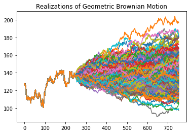
(Algorithm taken from the wikipedia page on GBM and from Hull, OF&OD 8th ed. §13.3)
¶ The predictive analytics sub-process
An example of parametric specification of the Equity Accumulator contract is below - it contains
- a reference to the underlying contract
- the algo trading rules
- formulas that are computed dynamically
- lookups of the historical prices of the underlying
- variables that are the subject of our investigation - we want to find the optimum combination
{
    "contract": "JPMC_NYSE",
    "file": "jpm.csv",
    "market": "NYSE",
    "desc": "...",
    "knock-in": "row.AdjClose > 145",
    "knock-out": "row.AdjClose <= 120",
    "dates": {
        "startdate": "2022-06-02",
        "enddate": "2024-05-22",
        "dateformat": "%Y-%m-%d",
        "filedateformat": "%Y-%m-%d"
    },
    "missing": "forward linear",
    "comments": [
       "BQ and SQ and PRESCRIPTIVE variables.",
       "the expressions can make use of min, max, avg, abs, math.ceil() et cetera.",
       "H is the historical time series."
    ],
    "buy": {
        "qty": "BQ",
        "at": "hist('AdjClose',T,0,H)",
        "when": "hist('AdjClose',T,0,H) > hist('AdjClose',T,-1,H)"
    },
    "sell": {
        "qty": "SQ",
        "at": "hist('AdjClose',T,0,H)",
        "when": "hist('AdjClose',T,0,H) < hist('AdjClose',T,-1,H)",
        "desc": "if 2% up or more, sell"
    }
}
The buy quantity and sell quantity above are expressed as parameters "BQ" and "SQ".
We will generate multiple scenarios based on random values.
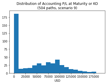
For our sample scenario #9, which comes with (BQ,SQ) = (6, 9), the distribution of the PV is as follows:
print('len:',len(sample_histog_data),'max:',max(path_lastCumCF))
# len: 504 max: 194444.43
pyplot.hist(path_lastCumCF, density=False, bins=[10000*i for i in range(20)])
¶ The histogram of P/L for the predicted scenario #9
For our scenario #9, (BQ, SQ) = (6, 9)
¶ Evaluation
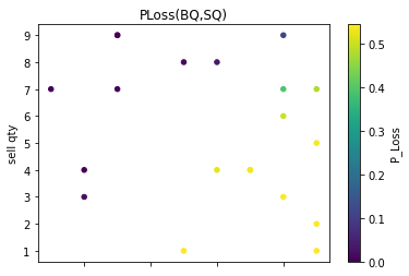
¶ The prescriptive analytics sub-process
The optimization of our objective (i.e., minimize the probability of loss) occurred, in our simulations, with these parameters:
| BuyQty | SellQty | P(Loss) | Max CumulCashFlow | Min CumulCashFlow |
|---|---|---|---|---|
| 2 | 4 | 0.0 | 50121.17 | 0.00 |
| 3 | 9 | 0.0 | 132204.52 | 0.00 |
| 1 | 7 | 0.0 | 120098.53 | 0.00 |
| 3 | 7 | 0.0 | 94189.34 | 0.00 |
| 3 | 9 | 0.0 | 132204.52 | 0.00 |
¶ Deployment
The python notebook (code and charts), is available at this link
The code ready for Ray parallel runs is available at this link
¶ Fitting the desktop code into a parallel computing framework
The non-parallel execution of 6 prescriptive scenarios,
each with 504 2-year stochastic future price paths,
takes approximately 2 hours 30 minutes on an AWS t2.micro EC2 instance.
The same code, having most of the computation that is an embarassingly parallel workload, can be easily transformed in a parallel code that sits on top of the python Ray framework and its Futures.
The same can be seamlessly deployed on AWS Glue that, since 2023, supports Ray in a few regions.
The list of the modifications to the python code are as follows:
lines added:
# GLUERAY
import ray
ray.init('auto')
decoration added in the function that runs as a parallel task, which is:
apply the financial contract rules (the version with the parameters defined by scenario S) to one 2-year future path price P
# GLUERAY
# By adding the `@ray.remote` decorator, a regular Python function
# becomes a Ray remote function.
@ray.remote
def get_remote_task_result(acchist_stats_dict,contract_dict,noFutprices,scn):
function execution modification:
    # GLUERAY

    # non-Ray:
    # scn_lastCumCF_array = [ get_remote_task_result(acchist.stats,contract_dict,noFutprices,scn) for pp in range(noPaths) ]

        # with Ray:
    scn_lastCumCF_array_futs = [ get_remote_task_result.remote(acchist.stats,contract_dict,noFutprices,scn) for pp in range(noPaths) ]
    scn_lastCumCF_array = ray.get(scn_lastCumCF_array_futs) # = waitAll API
The modified python script, wrapped in a glue job that we call "ray_kiko1", is executed with the following AWS CLI command:
aws glue start-job-run --job-name ray_kiko1 --number-of-workers 8 --worker-type Z.2X --region eu-west-1 --arguments='--pip-install="matplotlib,pandas"'
The parallel execution of 20 prescriptive scenarios,
each with 504 2-year stochastic future price paths,
takes approximately 6 minutes - of which 30 sec for start-up - with the 8 workers provided (16 DPUs).
Cost = USD 0.74 (updated 2023)
NB - the program is designed as a serial execution of scenarios that include the paraller evaluation of the 504 price paths.
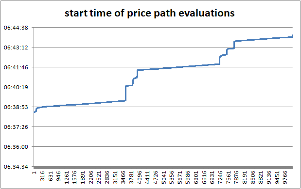
The telemetry is implemented as calls to an instance of nginx:
server:
image: "nginx:latest"
nginx.conf
log_format main '$time_local;$time_iso8601;$remote_addr;$status;$request';
python client:
payload={'tag':tag,'scenario':scenario,'pxpath':pxpath}
response = requests.head(http://aws-ec2-url/log, params=payload)
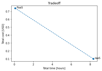
¶ Cost/time tradeoff
| service | computed scenarios | cost/hour | cost/job | hours | total cost |
|---|---|---|---|---|---|
| IaaS (AWS EC2) | 6 | 0.0116 | N/A | 2.50 | 0.03 |
| IaaS (AWS EC2) (projection) | 20 | 0.0116 | 8.33 | 0.10 | |
| Paas (AWS Glue) | 20 | N/A | 0.74 | 0.10 | 0.74 |
Costs in USD 2023
NB no lead time is included in EC2 calculations (EC2 setup time and final 'reduce' step takes less than 1 min)
¶ Conclusion
This case study addressed the optimization of a complex financial contract with respect to its risk profile.
The necessary analytical models were defined, and initial prototyping revealed significant computational demands.
A cloud-friendly technology was selected to enable scalable simulations with minimal redevelopment.
The final solution was implemented and executed successfully: we found the optimized contract and we identified a simple costing model established to balance performance and infrastructure expenditure.
¶ Appendix
¶ Relevant AWS and Ray links
- https://www.ray.io/
- https://docs.aws.amazon.com/glue/latest/dg/author-job-ray-job-parameters.html
- https://docs.aws.amazon.com/cli/latest/reference/glue/start-job-run.html
- https://docs.aws.amazon.com/glue/latest/dg/ray-jobs-section.html#author-job-ray-worker-accounting
- https://d1.awsstatic.com/events/Summits/reinvent2022/ANT343_Build-scalable-Python-jobs-with-AWS-Glue-for-Ray.pdf
¶
back to Portfolio
