¶ Summary
- A risk management system produces reports containing around one million records, each detailing key attributes of financial contracts along with risk sensitivities and P&L-Explain components. After system upgrades—whether in data or logic—the regenerated reports often show extensive differences: 30 columns across a million contracts can result in millions of changed cells. Although the changes appear large, the underlying root causes are suspected to be limited to a few key factors, making it essential to model and classify these differences and uncover shared characteristics among affected contracts.
- The goal is to define a method that can efficiently classify report differences and detect patterns or common properties across impacted contracts. The problem is reframed using Market Basket Analysis (MBA): each difference type (e.g., a PV change due to FX delta) is treated as an item in a “shopping basket,” and contract attributes (e.g., domestic currency = EUR) form the context—enabling pattern discovery similar to market shopping behavior analysis. From “People who buy diapers also buy beer” to "Trades with a significant change in the [MTD P/L impact due to interest rates] also happens to be bonds with a coupon payment date falling on the report generation date". This is a suggestion that there could be a bug in the calculation of the dirty price.
- The typical MBA implementation via the Naive Bayes algorithm, with its factorial complexity (O(N!)), proves impractical for datasets of this size. To address scalability, the problem is solved using the FPGrowth algorithm from PySpark’s MLlib—a big-data-capable, unsupervised machine learning approach. A mock report with fabricated differences is prepared to validate the method, and the algorithm is deployed and executed on AWS Glue for distributed processing.
- The algorithm successfully infers the underlying test rules within seconds, demonstrating both scalability and precision. This solution enables efficient classification of report differences, making it practical to trace large-scale discrepancies back to a small set of root causes.
¶ The execution process
Below are the links to the BPMN diagram that shows the entire process in which we create a mock report, we apply fabricated rules, we fit the model, we calibrate it and we verify the inferred rules.
→ full BPMN diagram edited with ARIS Express
¶ Preparation
¶ Baseline report generator
The implementation of the process mock data generator of the data-flow-diagram is based on the python Faker library and available here:
https://github.com/a-moscatelli/home/blob/main/am-wiki-assets/bayesdatamining/faker-datamining.py
¶ Generated baseline report
This is an excerpt of the CSV file generated by the process above.
The independent variables are the columns from 'trade_date' to 'delim'.
The dependent variables are the columns from 'delim' to '* PnL' (realized PnL, unrealized PnL, total PnL = R + U).
id,trade_date,  exp_date,          trader,tr_ccy,product,disc_curve,fx_cut,market,PnL_ccy,delim,uPnL,rPnL,PnL
 0,2023-05-04,2023-06-09,    Shannon Byrd,USDALL,fx swap,USDALL-GE,TKY1500,GE,USD,:,-7408923.84,-1466436.87,-8875360.71
 1,2023-05-14,2023-06-25,   Ashley Wilson,USDBWP,fx spot,USDBWP-GM,TKY1500,GM,USD,:,-5226084.9,-8085982.9,-13312067.8
 2,2023-04-29,2023-06-02,   Jasmine Baker,USDFJD,fx spot,USDFJD-AG,NYC1000,AG,USD,:,6394191.51,819916.38,7214107.89
 3,2023-05-14,2023-06-16,  Ashley Gilmore,USDAZN,fx futures,USDAZN-BW,TKY1500,BW,USD,:,7253124.02,-1717815.64,5535308.38
 4,2023-04-26,2023-05-13,Roberta Wade DVM,USDTMT,fx spot,USDTMT-WS,TKY1500,WS,USD,:,5089417.84,-8436149.32,-3346731.48
 5,2023-05-13,2023-05-14,  Jennifer Jones,USDZMW,fx fwd,USDZMW-GN,NYC1000,GN,USD,:,-9869409.75,-3996865.59,-13866275.34
 6,2023-05-11,2023-06-29,  Rebecca Flores,USDMNT,fx spot,USDMNT-GD,NYC1000,GD,USD,:,-996809.37,-8099321.43,-9096130.8
 7,2023-04-25,2023-06-02,  Stephen Murray,USDPAB,fx swap,USDPAB-OM,NYC1000,OM,USD,:,-3281707.89,797070.23,-2484637.66
 8,2023-05-02,2023-05-08,   John Franklin,USDLSL,fx futures,USDLSL-TH,TKY1500,TH,USD,:,6089738.13,2395105.79,8484843.92
 9,2023-04-28,2023-05-05,Jennifer Roberts,USDSRD,fx futures,USDSRD-SK,ECB1415,SK,USD,:,-5658173.72,-7390356.96,-13048530.68
¶ Execution
¶ Feature engineering (i.e. rule engine and signal derivation)
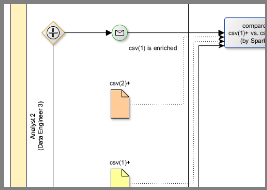
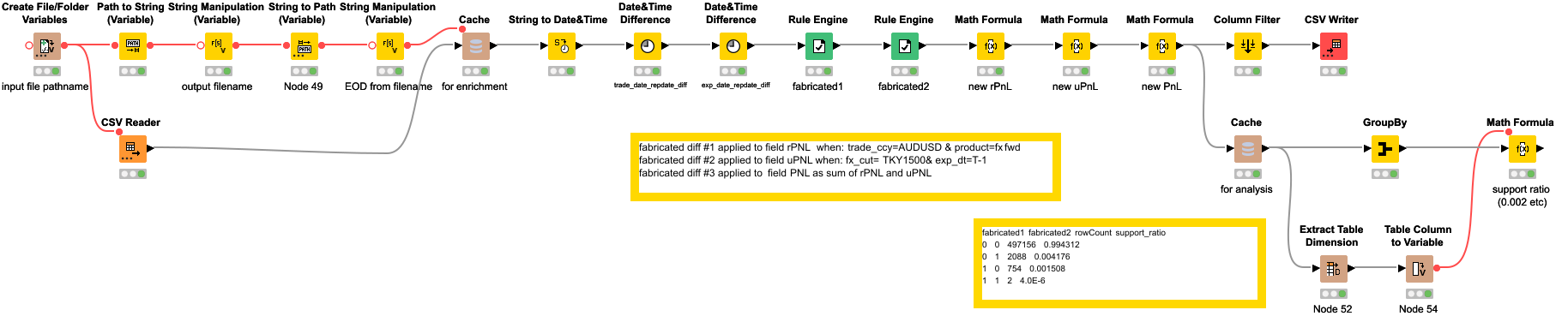
With the processes rule engine and signal derivation of the data-flow-diagram, we are going to generate the CANDIDATE report through the application of a few rules in order to get a set of fabricated differences. Then, we are going to calculate a few derived variables.
This step is done to transform our discrete variables (like the time_to_expire), into categorical ones (like expired_today true/false, expired_yesterday true/false), that are accepted by our data mining algorithm.
 Hi-res picture
After running the workflow above (see KNIME 4.6) we have a CANDIDATE report and the derived signals.
An example of signal expressions is as follows:
signal_1m = (expiry_date == report date - 1)
signal_1e = (expiry_date == report date)
signal_1p = (expiry_date == report date + 1)
signal_2p = (trade_date == report date + 1)
...
Providing these extra variables to the rule miner
is a way of verifying further hypotheses we have in mind:
is there any systematic issue with
the price computed for a class of trades expiring tomorrow?
¶ The data miner
In the process data miner we are running the FPGrowth provided with pySpark.
# docker
services:
    pyspark:
        image: "jupyter/pyspark-notebook:notebook-6.5.4"
FPGrowth is an enhancement of Apriori which is an enhancement of the Naive Bayes. It is an unsupervised machine learning implementation.
An example of Apriori implementation is available at:
https://github.com/a-moscatelli/DEV/tree/main/association_mining
The FPGrowth documentation supported by pySpark is available here
The FPGrowth requires the specification of a mininum support and confidence.
The minimum support we provide should be lower than the occurrence of the fabricated differences.
¶ Results
¶ Inferred rules
We now execute the process p3a of the data-flow-diagram.
Inferred rules for realized PnL: Jupyter notebook
| SN | antecedent | consequent | confidence | lift | support | lenA | lenC |
|---|---|---|---|---|---|---|---|
| 1 | [PnL_ccy=AUD, product=fx fwd] | [rPnL_diff=1] | 1 | 661.38 | 0 | 2 | 1 |
| 2 | [trade_ccy=AUDUSD, product=fx fwd] | [rPnL_diff=1] | 1 | 661.38 | 0 | 2 | 1 |
| 3 | [PnL_ccy=AUD, product=fx fwd, exp_date_m1=0] | [rPnL_diff=1] | 1 | 661.38 | 0 | 3 | 1 |
| 4 | [trade_ccy=AUDUSD, product=fx fwd, exp_date_m1=0] | [rPnL_diff=1] | 1 | 661.38 | 0 | 3 | 1 |
| 5 | [PnL_ccy=AUD, trade_ccy=AUDUSD, product=fx fwd] | [rPnL_diff=1] | 1 | 661.38 | 0 | 3 | 1 |
| 6 | [PnL_ccy=AUD, trade_ccy=AUDUSD, product=fx fwd, exp_date_m1=0] | [rPnL_diff=1] | 1 | 661.38 | 0 | 4 | 1 |
The implied rule 2 is exactly the rule that was applied to introduce fabricated differences.
The implied rule 1 is a byproduct of rule 2: in our input,
trade_ccy=AUDUSD ⇒ PnL_ccy=AUD
Inferred rules for unrealized PnL: Jupyter notebook
| SN | antecedent | consequent | confidence | lift | support | lenA | lenC |
|---|---|---|---|---|---|---|---|
| 1 | [exp_date_m1=1, fx_cut=TKY1500] | [uPnL_diff=1] | 1 | 239.23 | 0 | 2 | 1 |
| 2 | [exp_date_m1=1, fx_cut=TKY1500, PnL_ccy=USD] | [uPnL_diff=1] | 1 | 239.23 | 0 | 3 | 1 |
The implied rule 1 is exactly the rule that was applied to introduce fabricated differences.
The implied rule 2 is less general than rule 1 - but can still give clues about the root causes of the diffs.
¶ AWS test run
The rule mining script above,
executed on AWS Glue 3.0 with the default settings,
could process our half-million-record file pair
in 1 min 55 s
at a cost of USD 0.15
(Apr-2023)
aws glue start-job-run --job-name JOBNAME --region REGION --number-of-workers 10 --worker-type G.1X
:: default settings: 10 DPUs, G.1X
:: execution: 0.32 DPU hours
Full program: https://ampub.s3.eu-central-1.amazonaws.com/am-wiki-js/rulemining/FPG-FPmining-adapted-for-glue.py
Back to Portfolio
